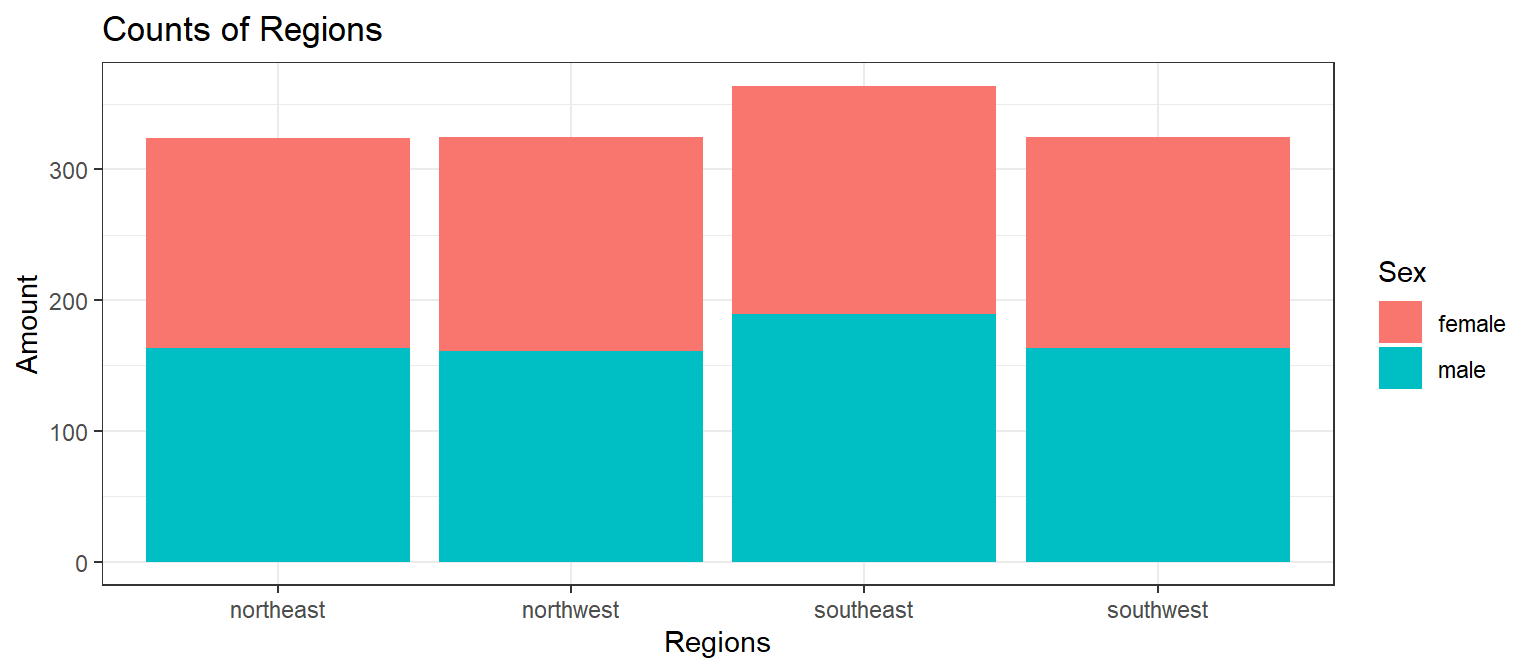
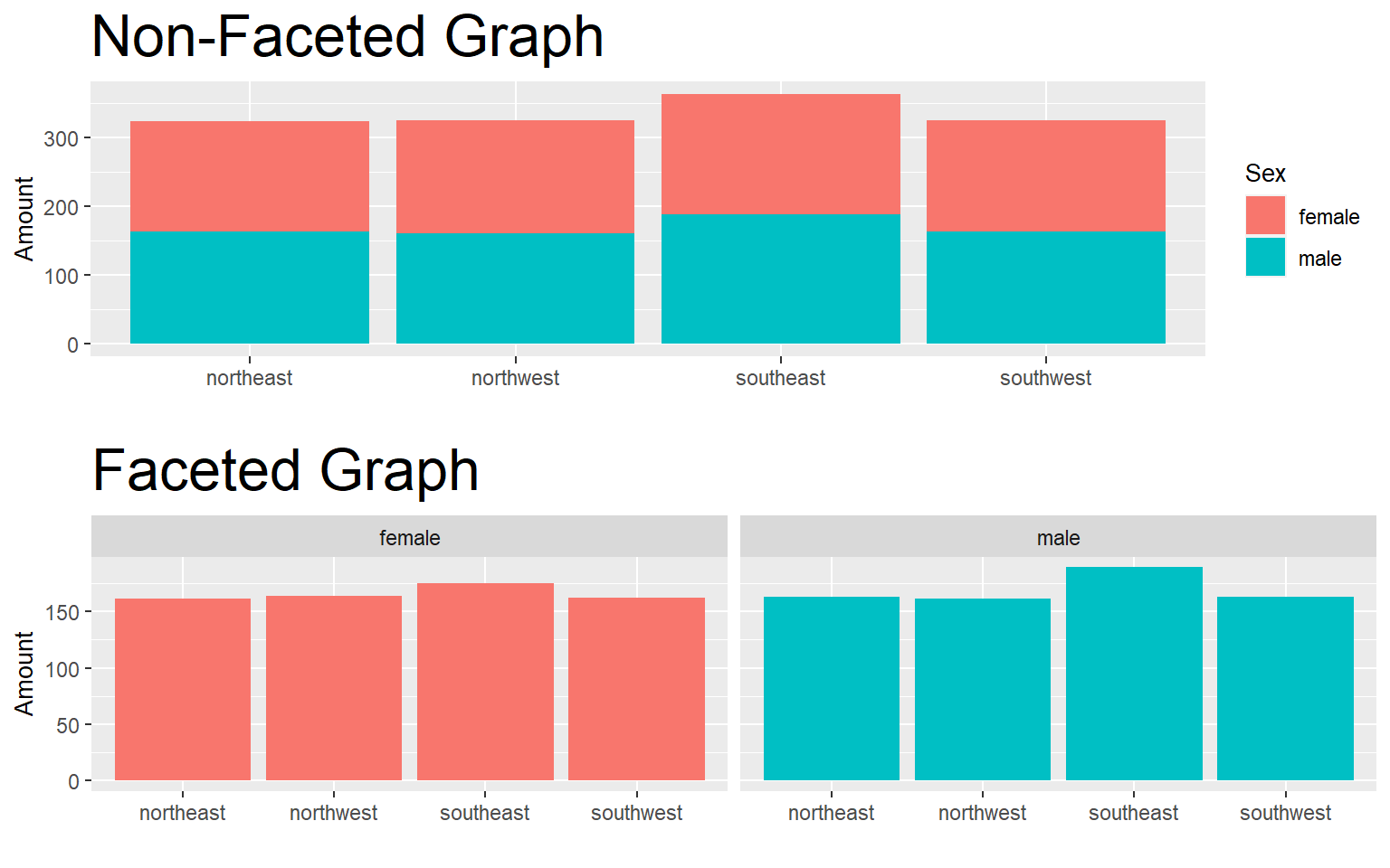
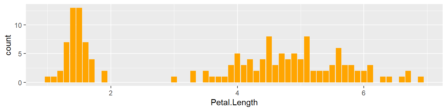
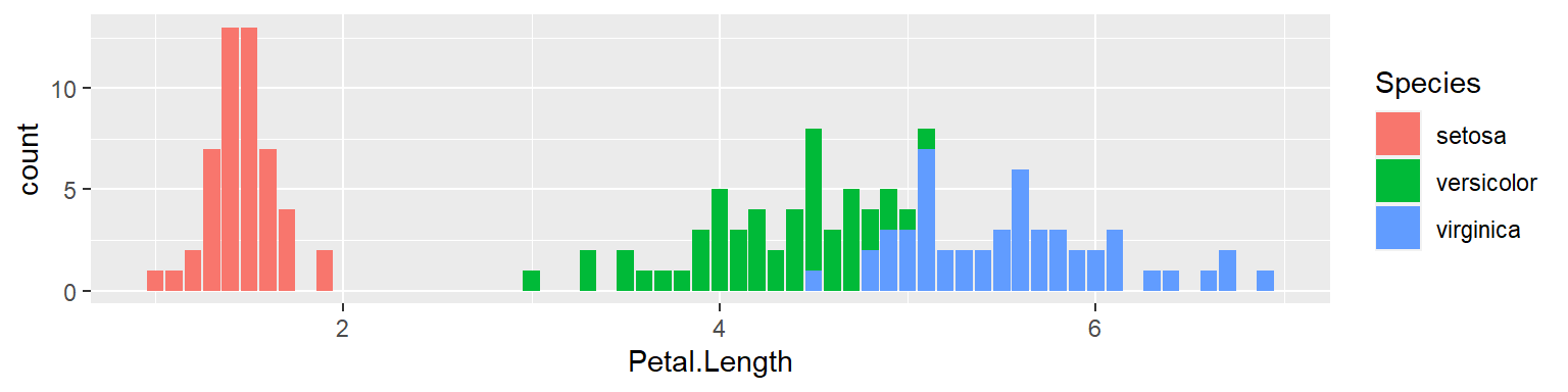
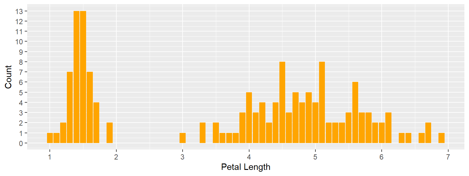
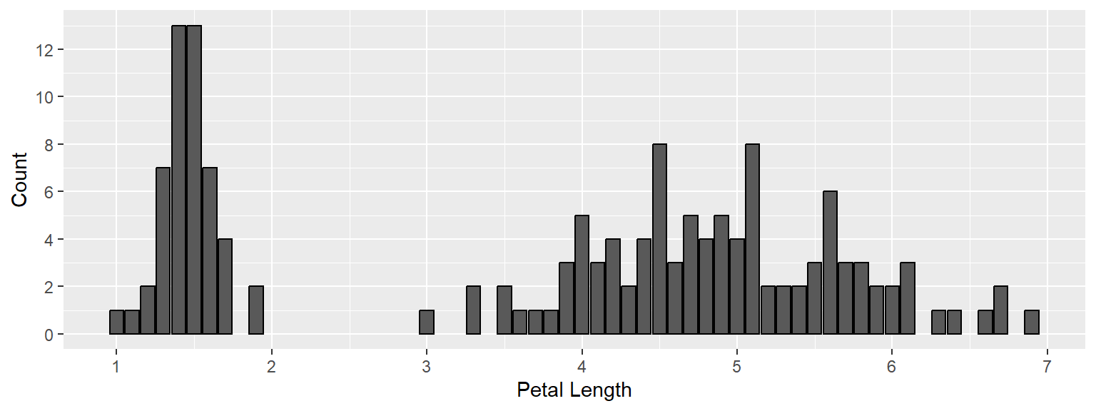
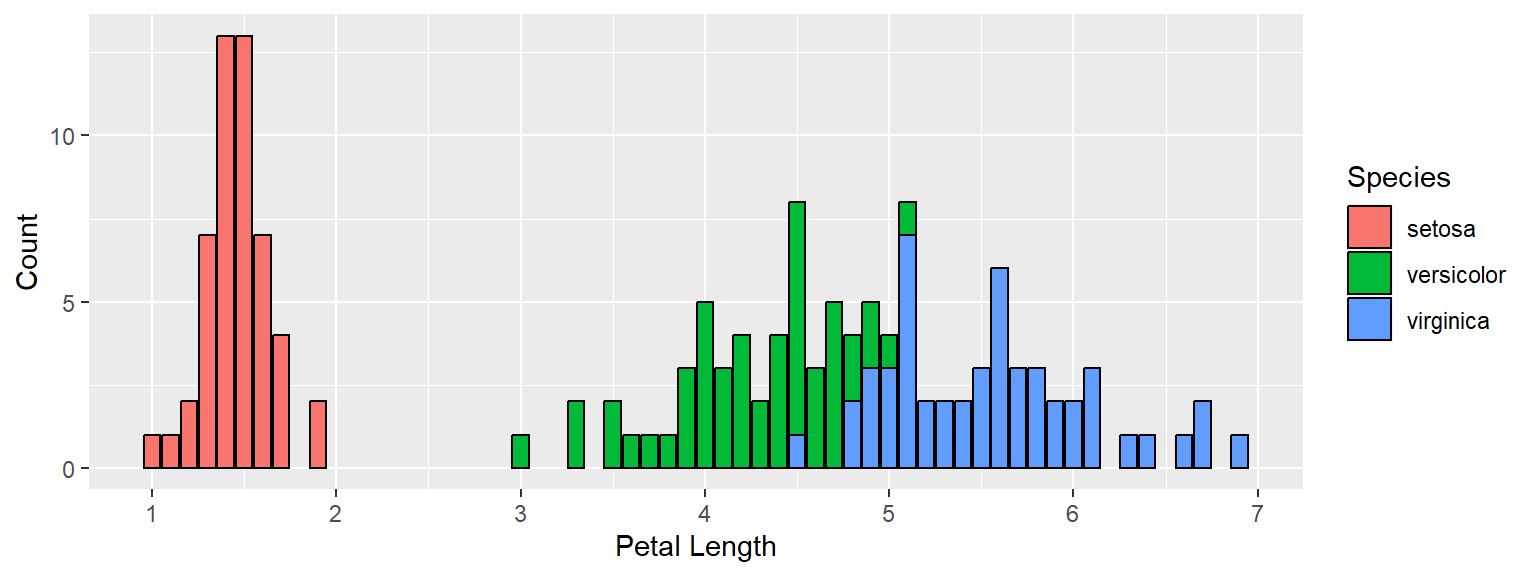
---title: "Lesson 06: Graphing Part 2"subtitle: Making graphs prettyimage: ggplot2.pngtoc: truefig-align: centerfig-width: 8fig-height: 3.5code-copy: truecode-overflow: wrapcode-line-numbers: truecode-fold: truecode-tools: trueeval: truemessage: falsewarning: false# toc: true---```{r}#| code-fold: false#| code-summary: "Data use in graphs below"library(tidyverse)dat <-read_csv("https://raw.githubusercontent.com/BrighamEaquinto/brighameaquinto.github.io/master/datasets/insurance.csv")```## Labeling #### `labs()`**Explanation**The `labs()` function is used to add label to the plot like the x-axis, the y-axis, and title. **Options**: - title - subtitle - caption - x - y**Example**```{r}ggplot(dat, aes(x = region, fill = sex))+geom_bar()+labs(title ="Counts of Regions", x ="Regions", y ="Amount", fill ="Sex")+theme_bw()```## Faceting### `facet_wrap()` & `facet_grid()`This of faceting as a third variable. - `facet_wrap()````{r}#| echo: false#| fig.height: 5color <-ggplot(dat, aes(x = region, fill = sex))+geom_bar()+labs(title ="Non-Faceted Graph", x ="", y ="Amount", fill ="Sex")+theme(title =element_text(size =20), axis.title =element_text(size =10), legend.title =element_text(size =10))facet <-ggplot(dat, aes(x = region, fill = sex))+geom_bar()+facet_wrap(~sex)+# facet_wrap(rows = vars(sex))+labs(title ="Faceted Graph", x ="", y ="Amount", fill ="Sex")+theme(title =element_text(size =20), axis.title =element_text(size =10), legend.title =element_text(size =10), legend.position ="none")ggpubr::ggarrange(color, facet, nrow =2)``````{r}#| code-fold: true#| code-summary: "Code"#| eval: falseggplot(dat, aes(x = region, fill = sex))+geom_bar()+facet_wrap(~sex)+labs(title ="Faceted Graph", x ="", y ="Amount", fill ="Sex")+theme(title =element_text(size =20), axis.title =element_text(size =10), legend.title =element_text(size =10), legend.position ="none")```## Themes The following theme options affect all the non-data aspects- `+ theme_bw()`- `+ theme_linedraw()`- `+ theme_light()`- `+ theme_dark()`- `+ theme_minimal()`- `+ theme_classic()`- `+ theme_void()`- `+ theme_test()`## Coloring#### AestheticIt is possible to set colors **dynamically** based on column of data or to set it as a **static** color. - `fill` and `color` inside aesthetic to a column of data- `fill` and `color` outside aesthetic to a static colorSetting colors dynamically and statically. ```{r}#| echo: false#| fig.height: 2tl <-ggplot(iris)+geom_bar(aes(x = Petal.Length), fill ="orange")tl``````{r}#| echo: false#| fig.height: 2tr <-ggplot(iris)+geom_bar(aes(x = Petal.Length, fill = Species))tr```:::{.callout-tip collapse="true"}## More Examples for Better Understanding::: columns::: {.column width="35%"}#### Case 1`geom_bar(aes(x = Petal.Length), fill = "orange")`- `fill` is set to 'orange' _outside_ the aesthetic - `color` is not used:::::: {.column width="3%"}:::::: {.column width="62%"}<br>```{r}#| fig.height: 3#| echo: falsetl <-ggplot(iris)+geom_bar(aes(x = Petal.Length), fill ="orange")+scale_x_continuous(breaks =c(0:20))+scale_y_continuous(breaks =c(0:20))+labs(x ="Petal Length", y ="Count")tl```::::::----::: columns::: {.column width="35%"}#### Case 2 `geom_bar(aes(x = Petal.Length), color = "black")`- `fill` is not used- `color` is set to 'black' _outside_ the aesthetic:::::: {.column width="3%"}:::::: {.column width="62%"}```{r}#| fig.height: 3#| echo: falsetm <-ggplot(iris)+geom_bar(aes(x = Petal.Length), color ="black")+scale_x_continuous(breaks =c(0:20))+scale_y_continuous(n.breaks =10)+labs(x ="Petal Length", y ="Count")tm```::::::----::: columns::: {.column width="35%"}#### Case 3`geom_bar(aes(x = Petal.Length), fill = "orange", color = "black")`- `fill` is set to 'orange' outside of the aesthetic- `color` is set to 'black' outside of the aesthetic:::::: {.column width="3%"}:::::: {.column width="62%"}```{r}#| fig.height: 3#| echo: falsebl <-ggplot(iris)+geom_bar(aes(x = Petal.Length), fill ="orange", color ="black")+scale_x_continuous(breaks =c(0:10))+labs(x ="Petal Length", y ="Count")bl```::::::----::: columns::: {.column width="35%"}#### Case 4You can do a combination of inside and outside of the aesthetic. `geom_bar(aes(x = Petal.Length, fill = Species), color = "black")`- `fill` is set to 'orange' _inside_ of the aesthetic- `color` is set to `Species` _outside_ of the aesthetic. Notice this is a column in the dataset, not a static color. :::::: {.column width="3%"}:::::: {.column width="62%"}```{r}#| echo: false#| fig.height: 3br <-ggplot(iris)+geom_bar(aes(x = Petal.Length, fill = Species), color ="black")+scale_x_continuous(breaks =c(0:10))+labs(x ="Petal Length", y ="Count")br```:::::::::## Scales ```{r}#| eval: falseggplot(iris, aes(Petal.Width, Petal.Length, color = Species))+geom_point()+scale_x_continuous(breaks =seq(0, 4, 1))+scale_y_continuous(breaks =seq(0,10,1))ggplot(mpg, aes(class, fill = class))+geom_bar()+# scale_x_discrete(limits = c("2seater"))scale_fill_manual(values =c("blue", "blue", "blue", "blue", "blue", "blue", "red"))# scale_x_continuous(# breaks = seq(15, 40, by = 5), # labels = , # limits = # )# scale_colour_brewer(palette = "Set1")# scale_colour_manual(values = c(Republican = "red", Democratic = "blue"))```<!-- ## Multiple Geoms## Other - colors - geom_text()/geoom_label() - labs() - themes() - legend - facet_wrap() - geom_boxplot() is often used with geom_jitter() to make powerful visualizations.- geom_bar() position argument- geom_jitter()- geom_text()- scales: - scale_x_continuous() - scale_y_continuous() - scale_colour_discrete()- ggsave("my-plot.pdf")```{r}base <- ggplot(mpg, aes(displ, hwy)) + geom_point(aes(colour = class))base + theme(legend.position = "left")base + theme(legend.position = "top")base + theme(legend.position = "bottom")base + theme(legend.position = "right") # the default```<br><br>## aes() Athestic- shape- size- color - alpha- linetype - groupshape, fill, color, size, stroke, linetype, alpha, group```{r}ggplot(iris, aes(Sepal.Width, Sepal.Length, color = Species, size = 10))+ geom_point(aes(shape = Species))+ geom_smooth(method='lm', aes(linetype = Species))``````{r}ggplot(iris, aes(Sepal.Width, Sepal.Length, size = 10, color = "red"))+ geom_point(aes(shape = Species))+ geom_smooth(method='lm', aes(linetype = Species))```## Coloring - the color and fill arguments are accepted inside the aes(). What about outside?- color is the boarder color- fill is the fill color- you can set hard colors or set it to a column in your dataset- R accepts color names in quotes and hex codes- `scale_fill_manual()`- `scale_color_manual()` -->